

Technical Drawing is one of the basic subjects in any engineering course. One could never overemphasize its importance. Ironically, it is often taken for granted – considered as a minor subject which is geared more to developing an engineer’s manual skill rather than his mental prowess. Thus, I will not be surprised if people, including engineers, would be intrigued by the article’s title and would ask: “Is there mathematics involved in Drawing?” I raised this same question once to my engineering students and the answer I got is: “yes, but only in scaling and dimensioning…” . Well, they’re partly right but they’re mostly wrong. Drawing is as mathematical as any civil engineering subject like say, geodetic surveying!
A drawing, the technical variety in particular, is nothing but a representation of a 3-dimensional object (with width, height and depth) and its location relative to the observer – into the two-dimensional realm of a flat surface, whether it’s the blackboard, a sketch pad or a computer monitor. Thus, going by this definition, drawing is essentially transforming the 3D coordinates of the corners of a real object into their 2D coordinates on the drawing surface, plotting these points and then connecting the dots with lines to represent the edges. To illustrate how point coordinate transformation is done from 3D to 2D, I could locate the hanging lamp in my room by its distance x from the side wall, distance y from the front wall and its distance z from the floor. However, in a perspective drawing of the room, the same bulb could be located in the sketch pad by defining the measurement u from the side and measurement v from the bottom of the sketch pad. Any other point inside the room could also be uniquely located in a similar fashion, transformed from its 3D location to its 2D position within the drawing frame.
Picture Plane and Orthographic Projections
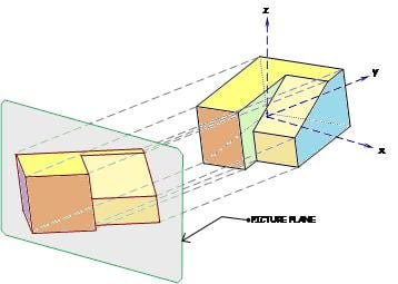
The picture plane is a very useful concept in the process of making technical drawings. By definition, It is an imaginary transparent plane that the observer sets between him and his subject so that the outlines and details of the object could be traced by projection. It might as well be a window, or a rectangle formed by the outstretched thumbs and forefingers of both hands like when you’re preparing to take a photo shoot.
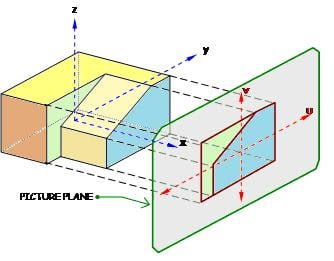
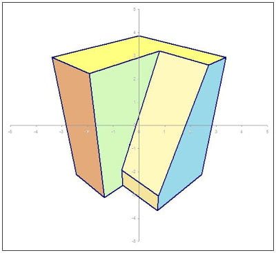
Figure 1 below shows a 3D solid, typical of building blocks or machine parts that we often encounter in engineering. If a picture plane is set directly in front of it, we could imagine parallel light rays reflected from the object to the picture plane allowing us to trace its “front view” as shown. Similarly, if the picture plane is transferred to the right of the object, a similar projection called the “right-side view” could be traced as in Figure 2. Now, notice that in both drawings, all corners of the object were projected to the picture plane but only a few of these show in the resulting drawings. That’s because some points are behind other points relative to the picture plane and thus, their projections would actually coincide with other points. This is what happens when you reduce the dimensions from three to two – the dimension normal to the picture plane is suppressed.

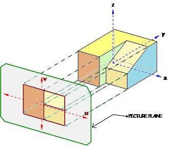

We may generalize, intuitively, that to reduce a three-dimensional object into its planar projection, we simply have to suppress the dimension normal to the picture plane. Thus, a point which is located at P(x,y,z) on three-dimensional space will plot as P(u,v) in the picture plane by a very simple transformation: (u,v) = (T).(x,y,z); where T is a transformation matrix converting the 3D coordinates into planar 2D coordinates.
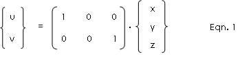
Explicitly for the “front view”, the y-coordinates are suppressed, thus any point located at (x, y, z) on space will now be plotted as a point (u,v) on the drawing pad. The conversion is done simply for each point as:

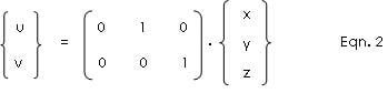
Similarly for the” right-side view”, the x-coordinates are also suppressed by using a different but similar transformation matrix:

We can derive a similar transformation matrix if you require a “top view” or any other view. Thus, we can go about placing the picture plane at any side and at any angle and inclination to obtain any side or angled view we want of the object so long as we can formulate the transformation matrix. Unfortunately, the transformation matrix is easily formulated only for cases where the picture plane is at right angles with the main axes of the object. For other angles and inclination, a rigorous expression is required.
But fortunately, there is an easier way. Instead of the observer going around the object, the observer and his picture plane could be fixed in one place, while we allow the object to rotate about any and all 3 axes! Thus, we can use the same 3D to 2D transformation matrix each time because we will be viewing it from a frontal picture plane all the time!
Coordinate Transformation through Rotations of Reference Axes
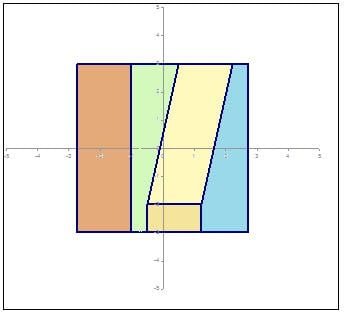
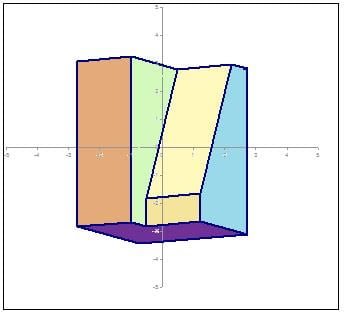
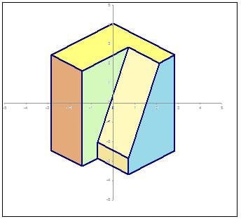
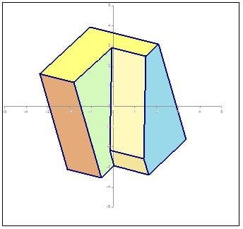
Suppose than from an initial upright and squared position we start rotating the object by angle A about the z axis, by an angle B about the x-axis and by an angle C about the y-axis; and then start measuring the new coordinates from the same set of axes as when the object is upright and squared. Then the object’s corners will have new coordinate triplets but essentially, the object has retained its shape. We can set-up the picture plane normal or perpendicular to the y-axis as before so that we can draw the projection simply by suppressing the y-coordinates using equation 1. Then we will be tracing its “front view” on the picture plane as usual – only that this time, the front view will be showing a different face.

Before we can do that however, we should be able to transform the coordinates of the object in its rotated state as in Figure 3. We start by considering a single point, P in space as shown in Figure 4. Its location in space is defined by the distances xo, yo and zo along the mutually perpendicular axes Xo, Yo and Zo respectively.

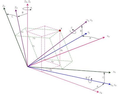
Notice from the above figure that the same point P could be as accurately located if it were referred from say the X3-Y3-Z3 set of axes. The distances x3, y3 and z3 could be taken as the original coordinates of the point prior to rotating the object. Our goal now would be to find a way of converting the triplet (x3, y3, z3) into its equivalent triplet (x0, y0, z0) so that the coordinates will be normalized with respect to the picture plane. Once it is normalized, we can use equation 1 to produce a frontal projection simply by suppressing the yo values.
To arrive at the X3-Y3-Z3 position from the Xo-Yo-Zo position, we first rotate the Zo axis by angle A to produce the X1-Y1-Z1 position; then we rotate the X1 axis by angle B to make the X2-Y2-Z2 position; and finally, we rotate the Y2 axis by angle C.
Let us take the rotations one by one.
Taking the Xo-Yo
plane after rotating the Zo axes by q as shown in Figure 5,
we can relate the triplets (x1, y1, z1) with (x0, y0, z0) by
simple trigonometry.

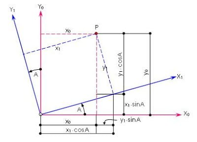
From the above figure, we can deduce:
xo = x1· cosA - y1· sinA
yo = x1· sinA + y1· cosA
zo = z1
which when written in matrix form becomes:

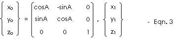
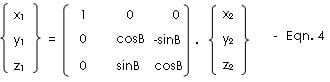
Similarly, we take the Y1,Z1 plane after applying a rotation angle B about the X1 axis as shown in Figure 6, below.

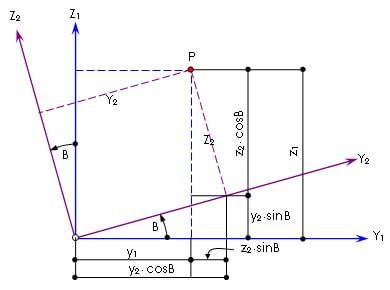
From which we can figure out the relationship:
x1 = x2
y1 = y2·cosB - z2·sinB
z1 = y2·sinB - z2·cosB
which in matrix form becomes:

Finally, we apply the rotation, angle C about Y2 axis to produce the X3-Y3-Z3 axes. Taking the x2-z2 plane as shown in Figure 7 below, we can derive the relationship as follows:

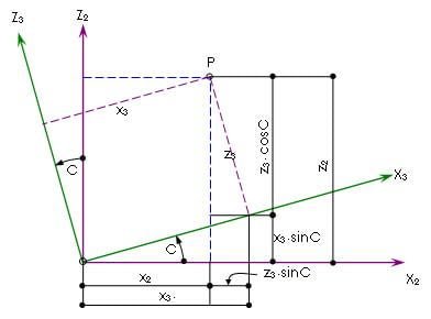
x2 = x3·cosC - z3·sinC
y2 = y3
z2 = x3·sinC + z3·cosC
which in matrix form becomes:

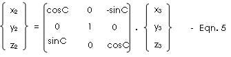
If we substitute Eqn. 5 into Eqn. 4; and then the resulting expression is substituted into Eqn. 3, we finally get the relationship between the Rotated Axes, (X3, Y3, Z3) and the Normal Axes (Xo, Yo, Zo).

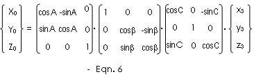
Thus, we have generalized the projection of any object whose orientation is defined by any combination of values of angles A, B, and C.
Physical Interpretation Of The Angular Values A, B, and C.
The angle, A is the Rotation or Turning Angle by which we rotate the object while we keep it upright. Varying the value of this parameter has the effect of allowing the observer to go around the object.
The angle, B is the Tilt Angle or Elevation Angle which tips the object forward or backward. Varying this parameter has the effect of allowing the observer to go over or under the object.
The angle, C is the Slant or the
Lean and measures the angle by which the object leans either
to the left or to the right. Varying the value of this
parameter is the equivalent of the observer’s tilting
his head on either side or for the photographer to shoot
with a diagonally held camera.
Now, its time to try our
little drawing algorithm. I have written a simple VB Program
which “reads” the coordinates of the object in
3D and the connectivity of the lines which defines the
edges. It then transforms these 3D coordinates into their 2D
counterparts. Using the transformed coordinates, it plots
the corners of the object on a window and then connect these
points with straight lines, establishing the shape of the
object in 2D. By varying the values of each angular
parameter A, B and C, we will be able to draw different
faces of the object.
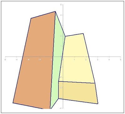
For example, if we wanted to draw
the Front View, we simply set the following parameters: A=0,
B = 0, and C=0

To draw the Right-Side View, we set the angular parameters
to:
A=-90, B = 0, and C=0

To draw the Top View, we set A = 0, B = 90, C = 0

If we set A = -30, B = 0, C = 0 then we obtain the Elevation View, from a horizontal vantage point 30 deg. to the right.

If we want a Worm’s View, from a vantage point 30 deg. to the right and 10 deg lower than the object, we should set A = -30, B = -10 and C = 0

Now, if we wanted to obtain the true isometric view, we have to turn the object to the left by 45 degress and make the object tilt forward by the arctan of (sin30/cos45) = 35.26 degrees and thus, the following parameters: A =-45, B = 35.26, C = 0

Why B = 35.26 degrees? I leave that as something for the reader to prove and ponder on.
Now, suppose that we are viewing from the same angles as in
the isometric position, how will the object appear to us if
we tilted our head by 15 degrees to the right. So then we
set
A =-45, B = 35.26 and C = 15

As you can see, this mathematical method is more powerful and far more versatile than the graphical method of projections which uses pen, paper, T-squares, triangles and straight edges. It also uses exactly the same technique and procedure whether one wants to draw a front view, a side view, a bottom view or an isometric view because in fact they are all Front Views being Frontal Projections of the object on Normalized Coordinates.
But, it doesn’t stop there! When we made our Frontal Projections, we assume that the projection rays are parallel. This is very nearly true when, the viewer is infinitely distant from the observed object or when the latter is of relatively small dimensions. Actually, in most cases, the projection rays are far from parallel – especially if the observer is relatively near the object.
Perspective Projections
Orthographic Projections are fine for Technical Drawings where it is important to have consistent dimensional scale of measurements. However, Orthographic Projections present images that are not as “realistic” as they actually appear to us. A more realistic image or drawing could be attained if we take into account the fact that the projection rays converges to the observer rather than stay parallel. To illustrate, suppose that we set the Picture Plane at a distance “a” from the object and that we stand along the same line at a farther distance, D. This set up is illustrated in plan and in elevation by the figures below:

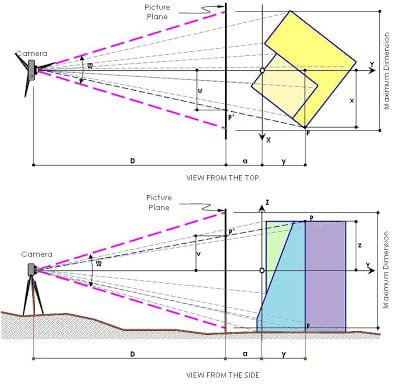
From the above figure, we chose a typical corner of the object which is labelled as P. Now observe how the image of P projects to the camera or eye of the observer along the blue dotted straight line which pierces the Picture Plane at point P’. In fact, all other points on the object project in an identical manner. Thus, the location of the plotted points on the picture plane is not only a function of the xo and zo coordinates (how far to the side and how high) but also yo (how far back). Using similar triangles:
u = (D)(x)/(D + a + y)
v = (D)(z)/(D + a + y)
we can rewrite this more concisely in transformation matrix format as:

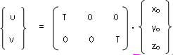
T = D / (D + a + y0)
which is identical in form to the Frontal Projection transformation (eqn. 1) but instead of 1’s we used the argument, T which is equal to
The View Angle and the View Distance
The human eye covers only a certain region at any one time. It can see only objects or parts of objects that fits within the “cone of vision”. The angle by which the cone of vision opens is called the View Angle, W. The wider the angle, the larger the coverage. To be able to see the entirety of an object, the observer has to be at a certain distance from the object so that the observed object fits within the cone. The distance is called the View Distance, D. The wider the View Angle, the less is the View Distance required. The relationship between View Distance and View Angle is defined by the equation
D = Smax / (2tan(W/2)) - a
where Smax is the maximum cross-sectional dimension. Since, the sizes of objects being viewed varies greatly, the View Distance also varies accordingly. Therefore, it is usually more practical and convenient to define the View Angle instead. Moreover, the view angle has more or less established values. For the normal human eye, W ranges from 30 to 60 degrees. For the lens of a standard camera the View Angle is about 50 degrees. Wide Angle cameras have lens angles of W = 90 to 180 degrees (fish eye lense). Macro as well as telephoto cameras have view angles usually less than 25 degrees. The distance “a” could be taken as zero, meaning that the picture plane is taken is placed within the object. More reasonably, we can place the PP just in front of the object by letting
a =1/2(xmax^2 + ymax^2 + zmax^2)^0.5
where xmax, ymax and zmax are the maximum dimensions in the x, y and z directions.
By changing the Transformation matrix of eqn.-1 to the Transfomation matrix of eqn.-7, we get Perspective Views rather than Orthographic Views.
I would also like to call your attention over the fact that the concept of a “Vanishing Point“, a fundamental concept in manually drawn perspective, has become totally irrelevant. Also, the mathematical method which was developed here do not make any distinction on one-point, two-point, three-point or multi-point perspectives – they are one and the same, depending on the orientation and view angle.
Thus, viewing the same object using a 50 degree view angle,W; A = -45, B = 35.26 and C = 0, we get this bird’s eye view perspective.

Using a wide-angle lens with W=150 deg and rotational parameters of A=-15, B = -15, C = 0, we get a dramatic worm’s eye view of a medium-rise building.

A normal view from the ground could usually be obtained by setting A = -50, B=-10, C=0 and W = 50 degrees as in the drawing below.
I used approximately the same angular settings A = -50, B=-10, C=0 with a 50mm lens camera to take the photograph of this majestic Our Lady Of Namacpacan Church in Luna, La Union.


So the next time somebody tells you that a graphic artist or a photographer knows nothing about Math, think again. He just might turn out to be a Math wizard.